Werner11.SpecialClass
Reading: BASIC RATEMAKING, Fifth Edition, May 2016, Geoff Werner, FCAS, MAAA & Claudine Modlin, FCAS, MAAA Willis Towers Watson
Chapter 11: Special Classification
Contents
Pop Quiz
Identify a data mining technique with the same name as the 4th planet of our solar system. Click for Answer
Study Tips
this section is not complete...
- territorial analysis of lesser importance
- ILFs important
- deductibles not important (easy, you can usually figure it out just knowing the basic formulas)
- size of loss for WC is not important
- ITV and coinsurnace important
BattleTable
Based on past exams, the main things you need to know (in rough order of importance) are:
- increased limits factors
- indemnity & coinsurance
reference part (a) part (b) part (c) part (d) E (2019.Fall #13) increased limits factors
- calculateE (2019.Fall #14) indemnity & coinsurance
- calculateindemnity & coinsurance
- equitable ratesindemnity & coinsurance
- adequate ratesE (2018.Fall #10) territory classes
- disadvantagesterritory classes
- creation ofE (2018.Fall #13) rate for AOI levels
-calculateunderinsurance
- problems withindemnity & coinsurance
- calculateE (2018.Spring #14) Excel Practice Problems E (2017.Fall #12) loss layers
- compare expected lossesincreased limits factors
- are they appropriate?increased limits factors
- calculation methodE (2017.Fall #14) indemnity & coinsurance
- coinsurance percentageindemnity & coinsurance
- ITV initiativesE (2017.Spring #11) rate for AOI levels
-calculateunderinsurance
- problems withindemnity & coinsurance
- calculateE (2016.Fall #11) increased limits factors
- calculateloss layer
- severity trendincreased limits factors
- comment on methodE (2016.Fall #14) indemnity & coinsurance
- coinsurance penaltyindemnity & coinsurance
- max coinsurance penaltyindemnity & coinsurance
- coinsurance ratiounderinsurance
- problems withE (2016.Spring #9) large deductible policy
- calculate premiumE (2016.Spring #11) increased limits factors
- calculateincreased limits factors
- impact of trendloss layer
- complement of credibilityE (2015.Spring #14) increased limits factors
- calculatedeductibles & limits
- loss elimination ratiodeductibles & limits
- pricing issuesE (2013.Fall #11) increased limits factors
- 2-dimensional data gridincreased limits factors
- std method vs. GLMincreased limits factors
- select & justifyE (2013.Fall #13) SCENARIO
- premium adequacy
Full BattleQuiz You must be logged in or this will not work.
In Plain English!
Territorial Ratemaking
Geography is a primary driver of claims experience and territory is a very commonly used rating variables. A insurer creates territories by grouping smaller geographic units such as zip codes or counties. An actuarial analysis then produces a relativity for each territory. The 2 steps in territorial ratemaking are:
- [1] establishing boundaries
- [2] determining relativities
Question: identify challenges to territorial ratemaking
- territory may be correlated with other rating variables
- (Ex: AOI and territory are correlated because high-value homes are often clustered)
- territories are often small so data may not be credible
Keep these challenges in the back of your mind while we look a little more closely at the details involved in establishing territorial boundaries.
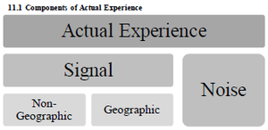
Step 1a in establishing territorial boundaries would be selecting a geographic unit, whether that's zip code or county or something else. Note that zip codes are easy to obtain but subject to change over time. Counties don't change but may be too large to be homogenous because they often contain both urban and rural areas. Werner and Modlin have a neat little diagram showing the components of actuarial experience.
What this diagram says is that the data, as we know, consists of signal and noise. (Hopefully more signal than noise) The signal can come from many different sources but we want to isolate the geographic signal. The non-geographic signal would be due to variables like age of home or marital status and would be dealt with separately.
Step 1b in establishing territorial boundaries would be assessing the geographic risk of each unit using internal data and also possibly external data like population density or rainfall. The geographic risk is expressed by a geographic estimator, which for a univariate method could be pure premium, but univariate methods don't work well here. They don't account for correlations with other rating variables and may give volatile results on data sets with low credibility such as individual zip codes. Multivariate methods are the better option because they are able to account for exposure correlation. They also perform better at separating signal from noise on data sets with low credibility.
Step 1c involves addressing credibility issues using a technique called spatial smoothing. If a particular zip code doesn't have sufficient credible data, we can supplement it by "borrowing" data from a similar nearby zip code. The goal is to get a more accurate geographic estimator for the original zip code or geographic unit by supplementing our analysis with similar data. There are 2 spatial smoothing methods:
- distance-based - weight the given geographical unit with units that are less than a specified distance away from the given unit
- → closer areas get more weight
- → works well for weather-related perils
- adjacency-based - weight the given geographical unit with units that are adjacent to the given unit
- → immediately adjacent areas get more weight
- → works well for urban/rural divisions and for natural boundaries like rivers or artificial boundaries like high-speed rail corridors
Step 1d is the final step and involves clustering the individual units in to territories that are:
- homogeneous
- credible
- statistically significant (different territories have statistically significant differences in risk and loss experience)
See Reserving Chapter 3 - Homogeneity & Credibility for a quick review. There are a couple of different methods for clustering:
- quantile methods - create clusters with an equal number of observations (Ex: geographic units) or equal weights (Ex: exposures)
- similarity methods - create clusters based on similarity of geographic estimators
These clustering methods don't necessarily produce contiguous territories. There could be zip codes in opposite corners of a state that have the same geographic estimator and grouped into the same territory even if they are hundreds of kilometers apart.
Question: identify a drawback of creating too few territories
- fewer territories means larger jumps in risk at boundaries (and potentially large jumps in rate)
Question: identify a drawback of creating too many territories
- more territories means each is smaller and therefore less credible (although with increasing sophistication of methods, some insurers are moving towards smaller territories)
The text doesn't go into any further mathematical details of creating territories. It is beyond the scope of the syllabus of this. Alice thinks you should be ready to give this exam problem a try:
- E (2018.Fall #10)
The quiz is easy...just a few things to memorize...
Increased Limits Ratemaking
Intro to Increased Limits
According to Werner
- Insurance products that provide protection against third-party liability claims usually offer the insured different amounts of insurance coverage, referred to as limits of insurance. Typically, the lowest level of insurance offered is referred to as the basic limit, and higher limits are referred to as increased limits.
In Pricing - Chapter 9 we learned how to calculate relativities for different levels of rating variables. Here we do the same thing for the rating variable policy limit but the method is more complicated.
Example A: Individual Uncensored Claims
Alice-the-Actuary's company offers auto insurance at 2 different policy limits: 50k and 100k. These are single limits. Let's call 50k the basic limit because that's the minimum limit that's offered. We assign this basic limit a relativity of 1.0. Then 100k is an increased limit and we want to calculate its relativity against the basic limit. Let's make up some fake data so we can see how this works.
Suppose you've got 2 customers with a basic limits policy and they've submitted claims as follows:
- claim #1: $2,000
- claim #2: $4,000
Then the average severity is obviously $3,000. Easy. But what if claim #2 were instead $60,000? Since the policy limit is 50k, this claim must be capped at $50,000 and the average severity is ($2,000 + $50,000)/2 = $26,000. Still easy, but this is why increased limits ratemaking is more complicated than what we covered in Pricing - Chapter 9. Sometimes that data base keeps the value of the original $60,000 claim even though only $50,000 would be paid out. But sometimes this extra information is lost. The data processing system would cap the claim at $50,000 before entry and the fact that it was originally a $60,000 claims is lost forever. This is also called censoring the data and when data is censored, we lose valuable information. Another complication with increased limits ratemaking is that data at higher limits may be sparse and cause volatility in results.
Anyway, if we return to the original claims of $2,000 and $4,000 and assume these are the only 2 claims in the data then the Limited Average Severity or LAS at the basic limit 50k is $3,000:
- LAS(50k) = $3,000
Let's suppose Alice's company also has a couple of high-class customers who have a policy limit of 100K and they submitted claims as follows:
- claim #3: $60,000
- claim #4: $70,000
The average severity for all 4 claims is $29,000:
- LAS(100k) = $29,000
And the Increased Limit Factor or ILF for the higher 100k limit is:
- ILF(100k) = LAS(100k) / LAS(50k) = $29,000 / $3,000 = 9.67
The formula is intuitively obvious. In general, if B denotes the basic limit and H denotes the higher limit then:
ILF(H) = LAS(H) / LAS(B)
In this example it was easy to calculate LAS(H) and LAS(B) but this isn't always the case. It depends very much how the data is stored in the database. If we simply had a listing of all uncensored claims, we could use the above method. Often however, claims are censored the policy limits and we'll look at an example of that further down.
Before moving on, there are a assumptions you should probably be aware of:
Assumption 1: The ILF formula above assumes:
- all underwriting expenses are variable
- the variable expense and profit provisions do not vary by limit
Assumption 2: Frequency & Severity
- frequency and severity are independent
- frequency is the same for all limits
Werner uses these assumptions to derive the ILF formula. You can read if you want to but it should be enough to be aware of the assumptions and know how to do the calculation. Note that customers who select higher policy limits when they purchase their policy often have lower frequency. That implies that frequency and severity are not independent. A possible reason is that customers who choose higher limits are more risk-averse (they are willing to pay more for insurance protection) and are likely to be more careful drivers.
Example B: Ranges of Uncensored Claims
Werner has a pretty good example of the procedure introduced in the previous example but instead of listing all uncensored claims individually, they are grouped into ranges. Take a few minutes to work through it then try the web-based problem in the quiz.
The first problem in the quiz is practice for the above example.
Example C: Censored Claims
| Friendly warning: For me, this is the hardest problem in the pricing material. I don't know why I had so much trouble with it. Once I figured it out and practiced it a bunch of times I was fine but it just took me a while to get there. |
In Example B, the database contained the full loss amounts related to each claim. The amount paid on each claim however depended on the policy limit of the claimant. In other words, the cap due to the policy limits was applied at the very end. Unfortunately, the database usually doesn't contain the full claim amount because the cap due to the policy limit is applied at the beginning. This is what it means to censor the claims. Information is lost and the procedure for calculating ILFs is more nuanced.
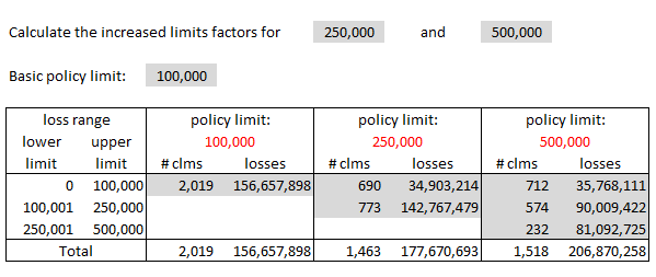
Let's see how to get from the uncensored data provided in Example B to the censored data for Example C as shown below. We'll need a little more information to do this. Example B had 5000 claims altogether but let's suppose that 2019 of these were on policies with a 100k limit. Since the claims are uncensored, you would also know how these 2019 claims fell into each range. Let's suppose the distribution is as shown in the table below. You now have enough information to calculate the censored losses for the 100k limit.
You take the losses as given for the 0→100k range but the losses in the higher ranges need to be capped at 100k. The censored losses for the 100k policy limit would be:
- $46,957,898 + $100,000 x (787 + 282 + 28) = $156,657,898
Without going into the remaining calculations, you do the same thing for policy limits 250k and 500k. (The text doesn't provide enough information to be able to do it. They just give you the final result.) The result is a 2-dimensional grid of count and loss information:
Anyway, below is my own version of the text example. I wrote out all the steps in Excel in a way that made sense to me. If you check my solution against the source text, you'll see they didn't actually complete the problem. They stopped after calculating the limited average severities but it was only 1 more simple step to get the final ILFs.
According to Werner, the general idea is as follows:
- When calculating the limited average severity for each limit, the actuary should use as much data as possible without allowing any bias due to censorship. The general approach is to calculate a limited average severity for each layer of loss and combine the estimates for each layer taking into consideration the probability of a claim occurring in the layer. The limited average severity of each layer is based solely on loss data from policies with limits as high as or higher than the upper limit of the layer.
You can refer to Werner for further explanation if you'd like but the best way to learn it just to keep practicing. I also found it helpful to sit in a dark room with my eyes closed and think really hard about the layout of the given information and how all the numbers fit into the solution. Anyway, here's how I did it. Study it and then do the practice problems. The quiz also has a web-based version for an infinite amount of practice.
Here are 4 practice problems in pdf format:
The second problem in the quiz is practice for the above example.
Miscellaneous ILF Topics
Here are few miscellaneous considerations regarding ILFs. They're easy. Just read them over.
- Development & Trending: Ideally, losses used in an Increased Limits Factor analysis should be developed and trended. Trending is important because recall from chapter 6 that trends have a leveraged effect on losses at higher layers. Development is important because different types of claims may develop differently. An example would be large claims versus small claims. Large claims may also have more volatility since it's more likely for courts to be involved if there is a dispute.
- Sparse Data and Fitted Curves: When performing an Increased Limits Factor analysis, empirical data as higher limits tends to be sparse compared to data at basic limits and this can lead to volatility in the results. One solution is to fit curves to empirical data to smooth out fluctuations. According to Werner:
- To calculate LAS(B), Limited Average Severity at the basic limit, just substitute B for H. Then ILF(H) = LAS(H) / LAS(B). You're unlikely to asked this on the exam, but memorize the formula just in case. It's a calculus exercise. Common distributions for f(x) are lognormal, Pareto, and truncated Pareto.
- Multivariate Approach: A multivariate approach to increased limits (such as GLMs) does not assume frequency is same for all sizes of risk and this is an advantage. For example, frequency may actually be lower for higher policy limits. This may be because customers who buy higher limits are more risk-averse and take other steps to mitigate losses. For that reason results are sometimes counter-intuitive. We could have H1 < H2 but ILF(H2) < ILF(H1). Just something to keep in mind.
The last few BattleCards in this quiz cover these concepts.
Deductible Pricing
Intro to Deductibles
A deductible is the amount the insured must pay before the insurer's reimbursement begins. For example if an insured has a collision causing $700 of damage and their policy deductible is $250, then the insured is responsible for $250 while the insurer pays the remaining $450 (subject to applicable policy limits.)
The $250 was a flat-dollar deductible, but the deductible can also be expressed as a percentage although this isn't common with auto policies. If a home insured for $300,000 has a 5% deductible then the insured would be responsible for the first $15,000 of loss. Easy.
Question: identify advantages of deductibles [Hint: PINC]
- Premium reduction (for insured)
- Incentive to mitigate losses (by insured)
- Nuisance claims are eliminated (insurer saves on LAE costs)
- Catastrophe exposure is controlled (for insurer)
The calculation problems on deductibles are easier than the problems on ILFs and have been asked far less frequently on prior exams. If you know the basic formulas you can usually figure out how to do the problem. This section should take much less time to study than the ILF section.
Example A: Given Ground-Up Losses
Deductible relativities are typically calculated using a loss elimination ratio or LER. If D is the deductible amount then LER(D) is the loss elimination ratio for deductible D. The text derives the following formula:
- LER(D) = (losses eliminated by deductible) / (ground-up losses)
The text derives this formula assuming all expenses are variable and that the variable expenses and profit are a constant percentage of premium. I don't think the derivation is important but keep in mind the assumptions. Once you've got the LER, calculating the deductible relativity is easy:
- deductible relativity = 1 – LER(D)
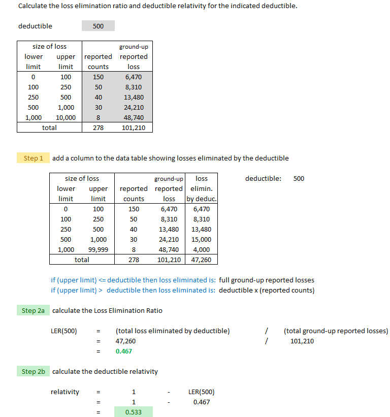
Below is an example Alice worked out that is similar to example from the text. A key observation is that you're given ground-up losses. That means if an insured has an accident causing $700 worth of damage and their deductible is $250, the insurer would record $700 of ground-up losses in their database even though they pay only $450 in net losses. It also means that if the accident caused only $200 worth of damage, the insurer would still record have a record of the $200 ground-up loss even though their net loss is nothing. This is similar to censored versus uncensored losses in the ILF procedure.
The first calculation problem in this quiz has a similar web-based problem for practice.
Example B: Given Net Losses
In the previous example you were given ground-up losses but this is often not available for deductible data. It was similar with ILFs. The ILF procedure was much easier when you had uncensored data versus censored data but it's more likely for an insurer's loss database to have only censored ILF data. With deductibles, the insurer likely records only net losses. For insureds with a deductible of $250, the insurer would have no idea how many accidents there were where the total damage was less than $250.
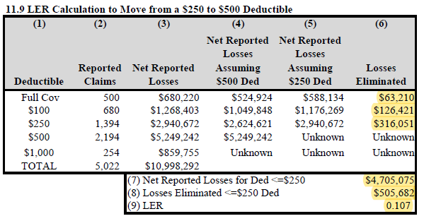
The example below is from the text and shows how to calculate the LER when moving from a $250 deductible to a $500 deductible.
Deductibles: to find losses eliminated when changing from deductible D1 to D2, use only data on policies with deductibles ≤ D1
For this example, this means we can only use data on policies with deductibles ≤ $250. The highlighted values are the only values you have to calculate. Everything else is given.
The second web-based problem in this quiz provides more practice calculating the deductible relativity when given net losses rather than ground-up losses.
Size of Risk for Worker's Compensation
Insurance to Value (ITV)
Full BattleQuiz You must be logged in or this will not work.
POP QUIZ ANSWERS
MARS or Multivariate Adaptive Regression Spline.
- The MARS algorithm operates as a multiple piecewise linear regression where each breakpoint defines a region for a particular linear regression equation.


