Werner12.Credibility

Reading: BASIC RATEMAKING, Fifth Edition, May 2016, Geoff Werner, FCAS, MAAA & Claudine Modlin, FCAS, MAAA Willis Towers Watson

Chapter 12: Credibility

Pop Quiz

Which of these are ITV (Insurance-to-Value) initiatives:

• insurers offer GRC (Guaranteed Replacement cost)

→ allows replacement cost to exceed the policy limit if the property is 100% insured to value

• insurers use more sophisticated property estimation tools

→ so insurers know more accurately whether a property is appropriately insured

• Ian-the-Intern brings you coffee when you get to work in the mornings

→ so you can examine policy forms with more energy and focus

Click for Answer 

Study Tips

VIDEO: W-12 (001) Credibility → 4:30 Forum

This chapter begins with some material on the theory of credibility that has already been covered extensively in prior exams. Since it's all review, you can get through the "Intro" section pretty quickly.

The new material for you is on methods for finding complements of credibility. There are a lot of them, 10 altogether, but the source text is well-organized and the wiki follows the organization of the text. Most of the methods are not difficult but Harwayne's method is an exception and you'll need to allocate a full day to learning it (not including review.)

The ranking table lists this chapter as Bottom 20% according to the average # of points it was worth on past exams. Credibility does come up however in many problems where you have to calculate an indication, but it's usually just a small part of the problem.

Desirable Qualities of a Complement of Credibility: The single most important thing to memorize is the list of 6 desirable qualities of a complement of credibility. Each of the 10 methods is then evaluated according to these 6 qualities but if you understand the methods, you don't necessarily have to memorize how each method performs individually. You can figure it out based on common sense. You should at least know however, what the best and worst methods are, and this is covered in the wiki article.

Complements of Credibility - First Dollar Methods: Harwayne's method hasn't often appeared on the exam, but when it did, it was worth a lot of points. That means that unless you are very pressed for time, you've got to take the time to learn it. And learn it solidly because it's very confusing and easy to mess up when you're under pressure on the exam. The method "Trended Present Rates" also comes up on the exam from time to time but it's much easier than Harwayne's method.

Complements of Credibility - Excess Methods: This is really getting down to material that is rarely asked. The last published question on this topic was (2014.Spring #7). The main things to memorize are the formulas for the 4 methods, then just do a few practice problems. The first 2 excess methods: ILA and LLA (Increased Limits Analysis and Lower Limits Analysis) are easy once you've practiced them a few times. The 3^rd method, LA (Limits Analysis) is somewhat more complicated. For the 4^th method on Fitted Curves, just memorize the formula. It involves integrals so you can't be asked to do a calculation on the exam, but they could create an essay-style question where you at least had to recognize and understand the formula.

Estimated study time: 3 days (not including subsequent review time)

BattleTable

Based on past exams, the main things you need to know (in rough order of importance) are:

• desirable qualities for a complement of credibility
• Harwayne's method - for calculating the complement of credibility
• trended present rates - for calculating the complement of credibility
• limits analysis - for calculating the complement of credibility

Let C of C stand for Complement of Credibility

reference	part (a)	part (b)	part (c)	part (d)
E (2019.Fall #3)	trended present rates - calculate C of C	C of C - first $ ratemaking
E (2019.Fall #12)	Harwayne's method - calculate C of C	current rate as C of C - advantages
E (2019.Spring #7)	Werner08.Indication	loss ratio method - credibility-weighted	disadvantage - using competitor rates
(2018.Spring #2)	See BA PowerPack
(2018.Spring #4)	See BA PowerPack
E (2017.Spring #9)	Harwayne's method - calculate C of C	Harwayne's method - appropriateness	C of C - desirable qualities
E (2015.Fall #3)	role of credibility - in ratemaking	C of C - desirable qualities
E (2015.Spring #11)	trended present rates 1 - calculate C of C
E (2014.Fall #8)	C of C - recommend	C of C 1 - use in indication
E (2014.Spring #7)	capped losses - calculate C of C in layer	limits analysis - calculate C of C in layer	limits analysis - disadvantages

¹ This problem is part of a much larger problem on calculating the indicated rate change.

Full BattleQuiz

In Plain English!

Introduction to Credibility

Necessary Criteria for Measures of Credibility

Intuitively, credibility is a measure of predictive value attached to a particular body of data. The necessary criteria for measures of credibility was covered on earlier exams but it doesn't hurt to review them quickly.

• Let Z a measure of credibility
• Let Y be number of claims

Then the 3 criteria (requirements) for a measure of credibility Z are:

• 0 ≤ Z ≤ 1
• Z is an increasing function of Y (first derivative of Z with respect to Y is positive)
• Z increases at a decreasing rate (second derivative of Z with respect to Y is negative)

You shouldn't be specifically asked to list these criteria on the exam but it's good to keep them in mind.

General Methods for Measuring Credibility

Classical Credibility

For classical credibility, the definition of full credibility is when:

• there is probability p that the observed value will differ from the expected value by less than k

We're going to skip the theoretical derivation and simply state the final formula for full credibility:

For example, if p = 90% and k = 0.05 then we look up (p+1)/2 = 95% on the normal distribution table. The value of 95% corresponds to a standard deviation of 1.645 so that

E(Y) = (1.645 / 0.05)² = 1,082

If the number of claims Y ≥ 1,082, then our data is fully credible and Z = 1.0. If Y < 1,082 then the formula for the credibility Z is the square root rule:

And if we had Y = 500, the result for our example is:

Z = (500 / 1,082)^½ = 0.680

Then our final estimate of of whatever quantity we're interested in is:

estimate (Classical)   =   Z x (observed value)   +   (1 - Z) x (related experience)

Part (a) of the follwing exam problem required you to do the above calculation to find to the credibility of the given data. It's part of a larger problem where you had to calculate the indicated rate change, but you should take a few minutes to do just the credibility part.

E (2019.Fall #3)

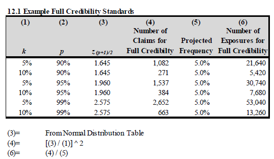
If you'd like a little more practice, here's a table from the text. You don't have to do the lookup on the normal distribution table but make sure you understand how to calculate columns (4) & (6). Note: Column (6) is for when exposures are used to define the full credibility standard instead of number of claims. In this case, you divide the numbers of claims by the frequency (as shown in the table.)

The last thing you need to know about classical credibility is...

Question: identify advantages (3) and disadvantages (2) of the classical credibility approach

advantages

• commonly used and generally accepted (by regulators)
• required data is readily available
• easy to compute

disadvantages

• makes simplifying assumptions (Ex: no variation in size of loss)
• doesn't consider quality of estimator compared to the latest observation and therefore judgment is required

Buhlmann

An important difference between Buhlmann and classical credibility is how the estimator is calculated. Instead of related experience, we substitute prior mean as shown below.

estimate (Buhlmann)   =   Z x (observed value)   +   (1 - Z) x (prior mean)

Of course, Z is calculated differently as well. It's less likely you'll be asked to use Buhlmann credibility on the exam, but you should know the formulas. Suppose

• N is the number of observations
• EVPV is the Expected Value of the Process Variance
• VHM is the Variance of the Hypothetical Mean

Then

• Z   =   N / (N + K)

where

• K   =   EVPV / VHM

As an incredibly simple example: (Even Ian-the-Intern thinks it's easy.)

• observed pure premium is $300 based on 55 observations
• EVPV is 2.50
• VHM is 0.40.
• prior mean is $280

Then

• K   =   6.25
• Z   =   55 / (55 + 6.25)   =   0.898

And our estimate of the pure premium is

• estimate (Buhlmann)   =   0.898 x $300 + (1 - 0.898) x $280   =   $298.0

And we'll finish up with this:

Question: identify advantages (1) and disadvantages (2) of the Buhlmann credibility approach

advantages

• generally accepted (less commonly used than classical credibility however)

disadvantages

• EVPV and VHM may be difficult to compute
• makes simplifying assumptions (Ex: risk parameters and risk process do not shift with time)

Bayesian

Bayesian credibility is not discussed in enough detail for you to be able to do the calculation. You do not calculate a Z-value. Instead, you use Baye's theorem to incorporate new information into the prior estimate.

Desirable Qualities of a Complement of Credibility

Recall the formula for the classical estimate from earlier:

estimate (Classical)   =   Z x (observed value)   +   (1 - Z) x (related experience)

Desirable qualities of a complement of credibility listed in the text pertain to related experience. Strictly speaking, the qualities listed below apply only when classical credibility is used. Buhlmann credibility is supposed to use the prior mean, but this is not always done in practice. Sometimes Buhlmann uses related experience. Anyway...

Question: identify desirable qualities for a complement of credibility [Hint: AU-SALE - Australian Sale - slip another shrimp on the barbie!]

• Accurate - low error variance around the future expected losses being estimated
• Unbiased - complement should not be routinely higher (or routinely lower) than the observed experience (which is different from being "close" to observed experience)

–

• Statistically independent from the base statistic - otherwise an error in the base statistic could be compounded
• Available - should be easy to obtain
• Logical relationship to base statistic - easier for a third party to understand (Ex: regulator)
• Easy to compute (so that even Ian-the-Intern can do it!)

Just memorize this list. You had to know it for the following 2 exam problems. You can take a look at them but you can't fully answer them yet because you need to know Harwayne's method for the first problem, and for the second problem, some knowledge of first-dollar methods for coming up with a complement of credibility from later in this chapter.

E (2017.Spring #9) part (c)

E (2015.Fall #3) Part (b)

And here's the introductory quiz.

mini BattleQuiz 1

Method for Developing Complements of Credibility: FIRST DOLLAR RATEMAKING

First dollar ratemaking is for products that cover claims from the first dollar of loss (or after some small deductible) up to some limit. Examples of first-dollar products are personal auto and homeowners. We generally use historical losses for the base statistic then select a complement from one of these 6 choices:

The first 2 methods don't come up very often:

• Loss Costs of a Larger Group that Include the Group being Rated
• Loss Costs of a Larger Related Group

These 3 methods tend to appear on the exam:

• Rate Change from the Larger Group Applied to Present Rates
• Harwayne’s Method
• Trended Present Rates

This method is terrible and is used only for new and/or small companies:

• Competitors’ Rates

Harwayne's method can be a little tricky. Trended present rates may require you to calculate trends or trend periods for losses which you can review by clicking the links. The other 4 methods don't generally require calculations as that would be given information. You just have to know when each is appropriate. You'll need to keep in mind AU-SALE, the desirable qualities of a complement of credibility.

Loss Costs of a Larger Group that Include the Group being Rated

Typical example: multi-state personal auto insurer uses countrywide data as a complement to the state being reviewed.

Countrywide data is higher volume thus more credible while still having a connection to the particular state. Let's evaluate countrywide data as a complement according to AU-SALE.

• Accurate?

→ probably not - if an insurer is active in many, there are likely real differences in loss costs between states so countrywide data would only be accurate if the state being reviewed is an "average" state

• Ubiased?

→ probably not - countrywide data will likely either be consistently high or consistently low unless the state being reviewed is an "average" state

• Statistically independent?

→ probably not - because the state being reviewed is part of the countrywide total - the bigger the state, the less independent

• Available?

YES! - because it's the company's own data

• Logical relationship to base

YES! - because countrywide data includes this state and the data is all from the same company

• Easy to calculate

YES! - there is nothing to calculate - the countrywide data should be available in the company's database

Loss Costs of Larger Group that Include the Base Group: scores 3 out of 6 desirable qualities - not a great method

Loss Costs of a Larger Related Group

Typical example: homeowners insurer uses "contents" loss data from house-owners to complement "contents" loss data for condo-dwellers

Loss experience for house-owners could be higher volume and more credible in a region where single-family houses predominate. House-owners and condo-owners are still related because they are both homes. Let's evaluate house-owners data as a complement according to AU-SALE.

• Accurate?

→ probably not - homeowners probably have more contents so loss experience would be different (higher)

• Ubiased?

→ depends - there likely is bias on the high side but if the bias is consistent, it can be corrected

• Statistically independent?

YES! - because house-owners data and condo-owners are separate

• Available?

→ depends - in this example it is available, but in general a larger related group may not be available

• Logical relationship to base

YES! - because it's a related group (same coverage, same company)

• Easy to calculate

YES! - there is nothing to calculate - the house-owners data should be available in the company's database

Loss Costs of Larger Related Group: scores 4 out of 6 desirable qualities (assuming depends counts for ½) - better than the previous method but still not great

Rate Change from the Larger Group Applied to Present Rates

Typical example: homeowners insurer uses "contents" loss experience rate change from house-owners to complement "contents" loss experience rate change for condo-dwellers

Did you spot the difference in the above example from the previous section. Both pertain to house-owners and condo-owners but here we use the rate change instead of the actual loss data. Using the rate change turns out to be a very good complement. Let's evaluate this complement according to AU-SALE.

• Accurate?

YES! - same coverage, same company, so likely to be accurate over the long-term assuming rate changes are relatively small

• Ubiased?

YES! - same coverage, same company, so over time the average rate change for house-owners is likely to be the same as for condo-owners

• Statistically independent?

YES! - because house-owners data and condo-owners are separate

• Available?

YES! - in this example it is available, but in general a larger related group may not be available

• Logical relationship to base

YES! - because it's a related group '(same coverage, same company)

• Easy to calculate

YES! - there is nothing to calculate - the house-owners data should be available in the company's database

Rate Change from Larger Group: scores 6 out of 6 desirable qualities - this is a very good method when used properly

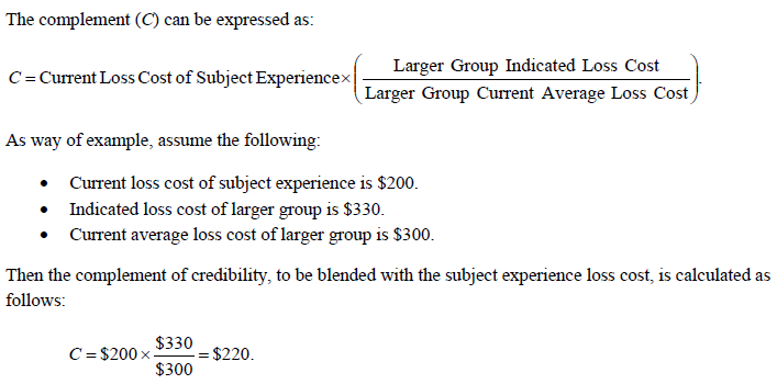
And here's a nice simple example from Werner:

Harwayne’s Method

Typical Example: Harwayne’s Method is used when the subject experience and related experience have significantly different distributions, and the related experience requires adjustment before it can be blended with the subject experience.

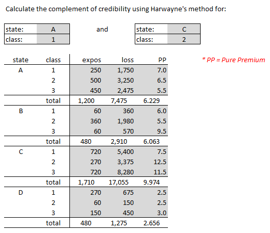
For Harwayne's method, we're first going to look at Alice's example and then evaluate it according to the 6 desirable qualities of a complement of credibility. Warning: It's very easy to get all discombobulated when doing Harwayne's method. Go slowly. Go carefully. You might even come up with a way organizing your solution that you like better than Alice's.

Here's the question. (Note that it's really 2 questions but using the same data)

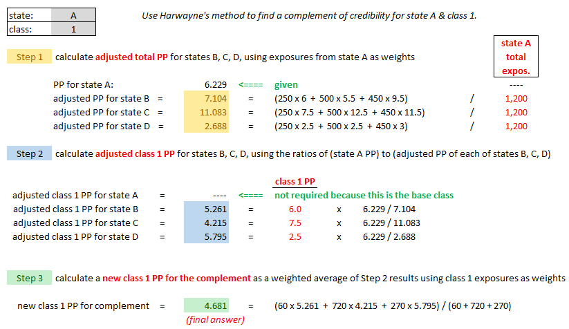
Here's the solution to the first question: State A, Class 1.

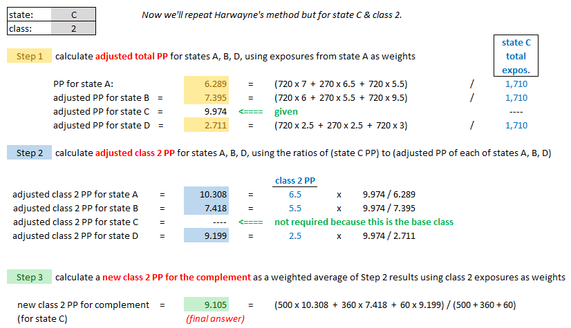
Here's the solution to the second question: State C, Class 2.

Ok, going through that was probably not a fun experience. Before I give you the practice problems, let's evaluate Harwayne's method as a complement according to AU-SALE.

• Accurate?

YES! - uses data from multiples segments so process variance should be minimized as long as volume in those segments is high enough

• Ubiased?

YES! - because it adjusts for distributional differences between classes

• Statistically independent?

YES! - base data and subject data come from different segments of data (even though it's the same company)

• Available?

YES! - usually available

• Logical relationship to base

YES! - but might be hard to explain because of the complexity of the method

• Easy to calculate

No - calculations are time-consuming and complicated

Harwayne: scores 5 out of 6 desirable qualities - Harwayne is almost as using the good as rate change from larger group applied to smaller group

Here are 2 practice problems just like the example. (It's really 4 practice problems altogether.)

Practice: 2 Harwayne's Method problems

Trended Present Rates

Typical example: when no larger group exists to use as a complement

The formula for the complement C is:

Now, we need to discuss the terms in this formula. It's a lot easier than Harwayne's method but you still have to be careful when applying it.

• present rate

- this is known because it's the "base"

- the present rate is being adjusted/trended to find a suitable complement for this base

• loss trend factor

- changes in cost levels may have occurred between the time the current rates were implemented and the time of the review

- this change has to be accounted for by trending the current rate

- for the trend period, use the original target effective date of the current rates for the "trend from" date

• (prior indicated loss cost) / (loss cost implemented with last review)

- this ratio is required because the implemented rate change is not always the same as the indicated rate change

- the complement should be based on the original indicated rate change and this ratio makes that adjustment

Once you have all the pieces, it's just a matter of substituting into the formula. You might need to review how to find the loss trend period. If so, just click the link in the previous sentence.

Here's a simple example. Suppose you're given:

• present average rate = $300
• selected loss trend = 4%
• indicated rate change from last review = 8%, and the target effective date was April 1, 2020
• implemented rate change from last review = 5%, and the actual effective date was May 15, 2020
• proposed effective date of next rate change is April 1, 2022

Then we calculate the complement using the above formula:

• C   =   $300 x (1.04)² x 1.08 / 1.05   =   $334

Note that to calculate the trend period of 2 years, we used the original target date and the proposed effective date. The actual effective date of the prior change is irrelevant. Let's evaluate trend present rates as a complement according to AU-SALE.

• Accurate?

YES! - provided current rates were based on high-volume data (so that process variance is low)

• Ubiased?

YES! - because pure trended costs are unbiased (i.e. no updating for recent experience)

• Statistically independent?

depends - unfortunately, "trended present rates" probably fails this test due to overlapping experience periods between the data current rates were based on the the data proposed rates are based on (maybe current rates were based on data from 2017-2019 and proposed rates are based on data from 2018-2020)

• Available?

YES! - unless your company has a very disorganized filing system the current rates should always be available :-)

• Logical relationship to base

YES! - obvious (it's related to the base by the above formula), and super-easy to explain to muggles like regulators :-)

• Easy to calculate

YES! - yup, pretty easy, if you remember how to calculate the loss trend period

Trended Present Rates: scores 5 out of 6 desirable qualities - PRETTY GOOD! - or maybe 5½ if depends counts for ½ because statistical independence might sometimes be satisfied

Competitors’ Rates

Typical example: new or small companies with small volumes of data often find their own data too unreliable for ratemaking.

Competitors likely have higher volume if they've been in existence for a longer period. The competitors’ data would then be more credible and have less process error but the only quality they possess from AU-SALE is Statistical independence.

There are many ways a competitor's data would not be appropriate for a complement. A competitor may have different U/W guidelines, mix of business, limits, deductibles, profit provision, and potentially others. In other words, it would not have a logical relationship to the base. It's a terrible method. New and/or small companies use it because they have no other choice.

Competitors' Rates: scores 1 out of 6 desirable qualities - a terrible method!

Method for Developing Complements of Credibility: EXCESS RATEMAKING

Excess ratemaking is different because data is often thin and volatile in excess layers. Since there tend to be very few claims in excess layers, predictions of excess losses attempt to use losses from below the attachment point. Werner discuss 4 methods for finding complements in excess layers:

• Increased limits analysis
• Lower limits analysis
• Limits analysis
• Fitted curves

Other challenges for excess ratemaking are:

• long-tailed lines such as liability where data develops slowly and immature data is less reliable
• inflationary effects because excess layers are affected differently versus total limits experience

Increased Limits Analysis

Typical example: data is available for ground-up losses through the attachment point "A"

Another way of saying this is: losses have not been truncated at any point below the bottom of the excess layer being priced

Conceptually, this formula adjusts losses capped at the attachment point to produce an estimate of losses in the specific excess layer.

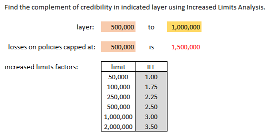
Here's an example problem. (There's another example in Werner plus some practice problems at the end of the Limits Analysis section.

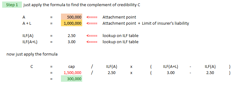
And here's the solution

Let's do a quick evaluation using AU-SALE:

• Accurate? not really - because to parameter error in selection of ILFs (not process error)

• Ubiased? no - because subject experience may have a different size of loss distribution than that used to develop the increased limits factors

• Statistically independent? somewhat - the error term of the complement is independent of the base statistic

• Available? depends - ILFs are required (could use industry factors) and ground-up losses that have not been truncated below the attachment point (might be harder to obtain)

• Logical relationship to base: not really - it's more logically related to data below the attachment point than to the limits being priced

• Easy to calculate: yes

Increased Limits Analysis does not seems like a very good method.

Lower Limits Analysis

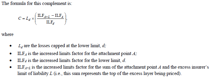
Typical example: when losses capped at the attachment point "A" are too thin to be reliable

The only difference between "Increased Limits Analysis" and "Lower Limits Analysis" is that LLA uses losses capped at a limit lower than the attachment point. We call this point d.

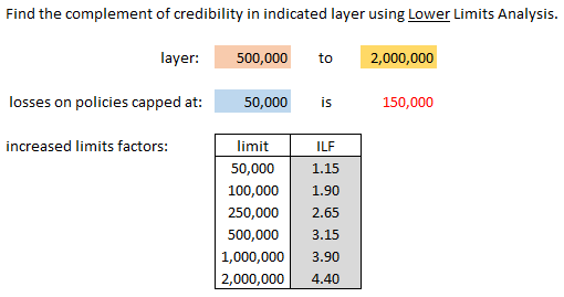
Here's an example problem. (There's another example in Werner plus some practice problems at the end of the Limits Analysis section.

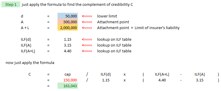
And here's the solution

Let's do a quick evaluation using AU-SALE:

• Accurate? not really - can't tell whether it's better or worse than ILA

• Ubiased? no - because subject experience probably has an even greater difference in size of loss distribution because losses are truncated at lower levels

• Statistically independent? somewhat - the error term of the complement is independent of the base statistic

• Available? depends - ILFs are required (could use industry factors) and ground-up losses that have not been truncated below the point d which is even lower than attachment point (might be harder to obtain)

• Logical relationship to base: not really - it's more logically related to data below the attachment point than to the limits being priced

• Easy to calculate: yes

Lower Limits Analysis does might be a little better than ILA (Increased Limits Analysis) but not by mch

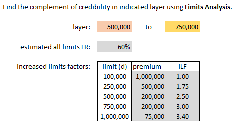
Limits Analysis

Typical example: when losses capped at a single point are not available

This is because:

Primary insurers sell policies with a range of policy limits. Some policies have limits below the attachment point; others above, and may even extend beyond the top of the excess layer.

Therefore, to calculate the complement...

...each policy’s limit and increased limit factor needs to be incorporated into the calculation.

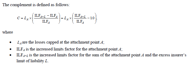
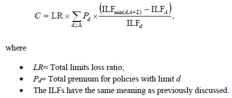
Here's the formula and notation according to Werner, but the formula makes the procedure look more complicated than it really is.

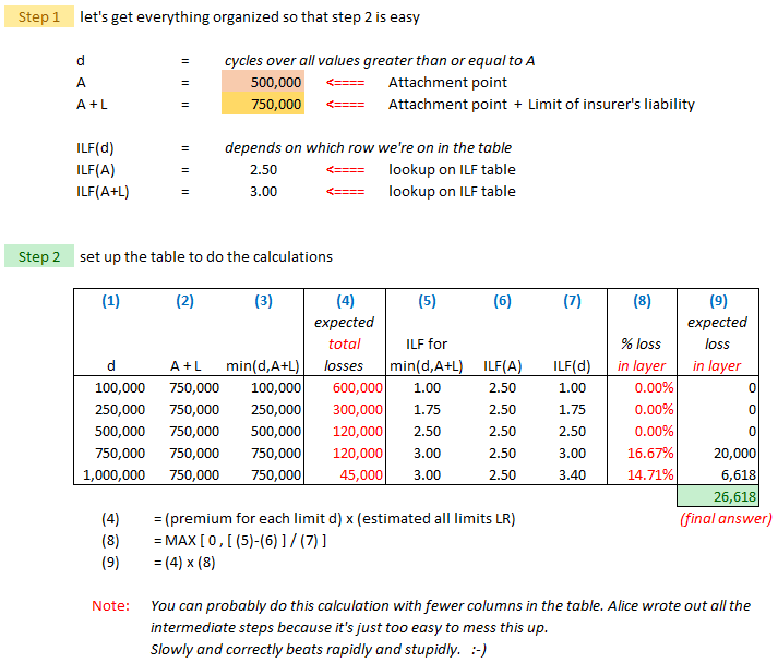
Here's the text example but Alice figured out a better way to organize it. You're welcome. :-)

Here's her solution. Please remember to thank Alice in your ACAS acceptance speech. :-)

Some thoughts on this procedure that may or may not be helpful...

LA (Limits Analysis) looks similar to the previous methods ILA and LLA, but there is a big conceptual difference. The previous methods are "1-step" methods - just pump up the basic limits loss to the range you want. But LA is "multi-step" in that it calculates SEGMENTS of the total loss then sums them. The thinking pattern when solving this problem is different. REMEMBER THIS!!!

Let's do a quick evaluation using AU-SALE:

• Accurate? not really - same as ILA and LLA, plus the additional (inaccurate) assumption that the loss ratio doesn't vary by limit

• Ubiased? no - same as ILA and LLA

• Statistically independent? somewhat - the error term of the complement is independent of the base statistic

• Available? depends - ILFs are required (could use industry factors)

• Logical relationship to base: not really - same as ILA and LLA - it's more logically related to data below the attachment point than to the limits being priced

• Easy to calculate: not really - it's time consuming and might be hard to explain to a regulator

Limits Analysis worse than ILA and LLA because of the additional loss ratio assumption, but without access to the full loss distribution it may be the only feasible method

Here's the last available official exam problem on this material:

E (2014.Spring #7)

And here are 6 more practice problems on "excess loss complement of credibility": 2 ILA problems, 2 LLA problems, 2 LA problems...

Practice: 6 Excess Loss Complement of Credibility problems

Fitted Curves

Typical example: when losses in excess layers are especially thin and volatile and a reasonable theoretical loss distribution can be found

The method of "fitted curves" is a little different from the other excess methods discussed in this chapter. The other methods used actual loss data but recall that data in higher layers is often thin and volatile. The "fitted curves" method generates its own data by fitting a curve to the actual data. This smooths out the volatility and hopefully makes the final results more reliable.

The text doesn't explain how to do the actual curve-fitting or show any example at all – it explains the procedure only in general terms and assumes you've already fitted a loss distribution f(x) to your data. Once you've got your distribution, you apply the following formula to find the percentage loss in each layer (A, A+L):

I'm not sure how much you really need to know about this, but just take a moment to look at the terms in formula. Intuitively:

% Losses in Layer (A, A + L)    =    [ $ Losses in Layer (A, A + L) ]    /    [ Total $ Losses ]

The denominator is the easiest to understand: It's the expected loss over the whole distribution. The first term in the numerator is the expected $-loss when the ground-up loss is between A and A + L. You have to subtract A to get the loss in the layer, then integrate from A to A+L. The second term in the numerator is the expected $-loss when the ground-up loss is greater than A+L. In this layer, the loss is capped at L and you integrate from A+L to ∞.

Anyway, once you've generated $-losses based on this distribution, you can use them just like you would real $-losses in the excess methods discussed earlier. (You would also need increased limits factors from somewhere.)

Let's do a quick evaluation using AU-SALE:

• Accurate? possibly - depends on how well f(x) fits the data

• Ubiased? probably - depends on how well f(x) fits the data

• Statistically independent? not so much - the curve-fitting procedure likely uses the same excess loss data as the as the base statistic

• Available? iffy - required data may not be readily available

• Logical relationship to base: yes - the curve-fitting procedure likely uses the same excess loss data as the as the base statistic (but this also works against statistical independence)

• Easy to calculate: NO! - it's computational complex and might be hard to explain to a regulator

Fitted Curves should produce reasonable-looking results if you've done the curve-fitting was done reasonably well

Summary

The appendices contain further examples of credibility. You can access the wiki articles for the appendices through the Ranking Table. Werner also makes a short comment at the end of the chapter about not mixing univariate and multivariate methods. He says that results from multivariate methods are not usually credibility-weighted with results from univariate methods. I'm not sure what you can do with that tidbit of information but it seemed like a tidy way to wrap things up!

mini BattleQuiz 2

Harwayne's method:

mini BattleQuiz 3

Trended Present Rates:

mini BattleQuiz 4

Misceallaneous:

mini BattleQuiz 5

Full BattleQuiz

POP QUIZ ANSWERS

Below are 2 of the 5 ITV initiatives from Pricing - Chapter 11 - Special Classification. Ian-the-Intern is not an ITV initiative.

• insurers offer GRC (Guaranteed Replacement cost)

→ allows replacement cost to exceed the policy limit if the property is 100% insured to value

• insurers use more sophisticated property estimation tools

→ so insurers know more accurately whether a property is appropriately insured

And the other 3 from Pricing - Chapter 11 - Special Classification are:

• insurers educate customers:

→ coverage is better if F/V is closer to 100% (for both insurer and insureds)

• insurers inspect property and use indexation clauses

→ more information allows insurers to better price a policy

→ indexation clauses ensure the face value of a policy keeps up with the value of the home

• insurers use a coinsurance clause

→ assigns a penalty if the coinsurance requirement is not met

Go back