Werner14.Implementation

Reading: BASIC RATEMAKING, Fifth Edition, May 2016, Geoff Werner, FCAS, MAAA & Claudine Modlin, FCAS, MAAA Willis Towers Watson

Chapter 14: Implementation

Pop Quiz

Do you remember the difference between a hard market and a soft market? Click for Answer 

BattleTable

Based on past exams, the main things you need to know (in rough order of importance) are:

• base rate - calculating the appropriate base rate to be implemented with a rate change
• territorial relativities calculating territorial relativities to be implemented with a rate change
• non-pricing solutions - bringing the Fundamental Insurance Equation into balance

reference	part (a)	part (b)	part (c)	part (d)
E (2018.Fall #12)	PP method (adjusted) - see Chapter 9 - Adj. PP	base rate - calculate	rating variable criteria - see social criteria
E (2017.Fall #13)	territorial relativities - calculate
E (2017.Spring #10)	U/W profit - calculate	base rate - calculate	base rate - evaluate mgmt suggestion
E (2016.Spring #12)	change in premium - calculate average	change in premium - distortion	non-pricing solutions - for inadequate rates
E (2015.Fall #9)	territorial relativities - revenue-neutral change	territorial relativities - evaluate impact
E (2015.Fall #11)	base rate (ext. of expos.) - calculate (see here)
E (2015.Spring #10)	territorial relativities - calculate	non-pricing solutions - for inadequate rates
E (2014.Spring #10)	deviation from indicated - 3 reasons	non-pricing solutions - for inadequate rates	base rate - calculate
E (2013.Fall #9)	territorial relativities - calculate
E (2013.Spring #14)	capping rates - identify issues	capping rates - reasons for

Full BattleQuiz

In Plain English!

Example Imbalance

Recall the Fundamental Insurance Equation:

   premium    =    (Losses   +   LAE   +   U/W Expenses)   +   U/W profit

If the premium on left side of the equation is projected to be $235, but the losses, expenses, and profit on right side of the equation are projected to be $250, then the equation is out of balance. The insurer would lose an average of $15 for each policy sold. Obviously that's a problem. In this chapter, we'll address that problem using both pricing and non-pricing solutions.

Non-Pricing Solutions

Non-pricing solutions attempt to reduce the costs on the right side of the Fundamental Insurance Equation. There are 4 terms on the right so that provides 3 options:

• reduce losses

→ tighten U/W requirements to eliminate policies that are underpriced

→ reduce coverage levels (Ex: reduce limits or insert coverage exclusions)

→ implement better loss controls (Ex: safety programs for WC)

• reduce LAE

→ Ex: reduce staffing levels in claims department

• reduce U/W expenses

→ Ex: reduce agent commission

You should memorize this list of non-pricing solutions. (Note that reducing the profit provision would be considered a pricing solution.)

mini BattleQuiz 1

Pricing Solutions

A pricing solution to an unbalanced Fundamental Insurance Equation is to adjust rates (versus losses or costs). In the example above, the average rate would need to be increased by $15 from $235 to $250. If this cannot be done, or if the company chooses not to do this, the U/W profit on the right side of the equation would automatically be $15 lower. Often a company may do a combination by raising rates less than the full $15, the difference being made up by a corresponding reduction in U/W profit.

Calculating New Rates for an Existing Product

Intro: The Rating Algorithm

The source text provides a list of 5 steps for calculating a final set of rates for an existing product. It probably isn't something that would be asked on the exam, but it's good to have a general idea of how it's done. I underlined the key action in each step as a memory hook. The first 3 items were covered in earlier chapters. (Note that item 2 regarding the rating algorithm is from chapter 2, which isn't on the syllabus.)

• Select an overall average premium target for the future policy period
• Finalize the structure of the rating algorithm
• Select the final rate differentials for each of the rating variables
• Calculate proposed fixed expense fees and other dollar additives, if applicable    ← major topic in this chapter
• Derive the base rate necessary to achieve the overall average premium target    ← major topic in this chapter

The examples in this chapter use the following example rating algorithm:

Rating Algorithm (average premium):    Pp   =   [ Bp x R1p x R2p   x   (1.0 – D1p – D2p) ]   +   Ap

where

• P_p = average premium per exposure
• B_p = base rate (proposed)
• R1_p, R2_p = relativities for rating variables 1 & 2 (proposed)
• D1_p, D2_p = discounts (proposed)
• A_p = additive expense fee (proposed)

As an incredibly simple example for Ian-the-Intern, let's use this formula to calculate the average premium given the following:

• B_p = $500
• R1_p = 1.1, R2_p = 1.15
• D1_p = 10%, D2_p = 5%
• A_p = $25

Simple substitution yields P_p = $562.63. If this were auto insurance, the discounts might have been something like 10% for airbags, and 5% for an anti-theft security for a security system.

There is a slightly different version of the rating algorithm that's also used in this chapter. Recall that P_p = P_p / X so if you multiply both sides of the formula by exposures X, you get:

Rating Algorithm (TOTAL premium):    Pp   =   [ [ Bp x R1p x R2p   x   (1.0 – D1p – D2p) ] + Ap ]   x   X

We will use this formula for total premium with the extension of exposures method for calculating a proposed base rate. If you check the source text, you'll see that their rating algorithm is written a little differently. Their formula looks more complicated because they included all of the subscripts. Strictly speaking, the subscripts should be there but I found it unnecessarily confusing to type them out every time. Let's just agree the subscripts are there even if they aren't specifically written. Very quickly, here's the text version:

If R1 (Rating Variable 1) has 3 different levels then i can take on the values 1,2, or 3. If R2 has 4 different levels, then j can take on the values 1,2,3 or 4. Same idea for the discounts D1 and D2 using the indices k and m. Note that "l", which is a small "el", is not used. This is to avoid confusion because it looks too much like the numeral "1".

Example A: Proposed Fixed Expense Fee

We're going to build to a more general example than the one presented in the text. First we need a couple of definitions:

definition: the variable premium is the portion of the total premium that varies by risk characteristics

definition: the additive premium is the portion of the total premium derived from expense fees and other dollar additives

* Additive premium is the same thing as flat premium.

Our rating algorithm incorporates fixed expenses through an additive per exposure expense fee A_p. How do we calculate this additive fee? The first example in Werner is super-simple and demonstrates the concept. Suppose we're given:

• E_F = average fixed expense per exposure = $20
• V = variable expense provision = 15.0%
• Q_T = target profit percentage = 5.0%

Then the premium we need to charge to cover this is:

• E_F / (1 - V - Q_T)   =   $20 / (1 - 15.0% - 5.0%)   =   $20 / 0.8   =   $25

This is the same adjustment as in chapters 7 and 8 when we adjusted the total loss cost to derive the average premium charged. Click to review the Pure Premium Formula. Recall also that the denominator (1-V-Q) is called the Variable Permissible Loss Ratio or VPLR.

The second example in Werner is almost as simple but instead of giving you E_F directly, they provide:

• F = fixed expense ratio = 8.0%
• P_p = projected average premium per exposure = $250

So you have to calculate E_F yourself:

• E_F   =   F x P_p   =   8.0% x $250   =   $20.

That gets you back to the starting point for the first example.

Here is a more realistic version of this type of problem:

And here are a couple of practice problems just like the example above...

Practice: 2 Fixed Expense Fee problems

Example B: Base Rate - Easy Version (No Rate Differential Changes)

Recall the 5 steps from the Intro for calculating a final set of rates for an existing product. The last step is:

• derive the base rate necessary to achieve the overall average premium target

We're going to look at several examples of how to do this starting with an easy example. First recall the rating algorithm as shown below. Having this formula (using either subscript "p" for proposed premium or subscript "c" for current premium) will make it clear what's happening algebraically:

P_p   =   [ B_p x R1_p x R2_p   x   (1.0 – D1_p – D2_p) ]   +   A_p

Of course, this formula also holds for current rates:

P_c   =   [ B_c x R1_c x R2_c   x   (1.0 – D1_c – D2_c) ]   +   A_c

Scenario B1: Assume we know B_c and P_c. We want to calculate the proposed base rate B_p that will achieve the proposed premium P_p. For this very simple scenario, we also make these assumptions:

• all premium is variable

→ A_p = A_c = 0

• rate differentials are not changing

→ R1_p = R1_c

→ R2_p = R2_c

→ D1_p = D1_c

→ D2_p = D2_c

If you substitute into the equations for P_p and P_c, cancel terms, then solve for B_p, you get:

Bp = Bc x (Pp / Pc)

This is so simple, you can just make up your own example. All that's happening is that the current base rate B_c is being increased by the same proportion as the increase in average premium.

Scenario B2: Same as scenario B1 except we allow the fixed expense fees A_p and A_c to be non-zero. If you again start with the above formulas for P_p and P_c then simple algebra yields:

Bp = Bc x (Pp – Ap) / (Pc – Ac)

As an example, suppose a 3.0% overall change is desired. One way of doing this is to increase both the base rate and fixed expense fee by 3.0%. But if you want to keep the (non-zero) fixed expense at the same level, the base rate increase would have to be greater than 3.0% to compensate. For example, if:

• P_c = 400
• P_p = 400 x 1.03 = 412
• B_c = 300
• A_p = A_c = 20

then

• B_p = 300 x (412 - 20) / (400 - 20) = 309.47

which is a 3.16% increase in the base rate.

Example C: Base Rate - Extension of Exposures

Examples C, D, E show how to calculate the new base rate when relativities are changing. Example C uses the extension of exposures method which is the most accurate because it rerates individual policies. The disadvantage is of course that it requires detailed policy level detail and that may not be readily available.

The example of the extension of exposures method from the source text is okay but it's presented in a way that makes it seem a lot more complicated than it really is. It starts on page 268 and you can take a look at it if you want but I decided to focus more on an old exam problem that uses this method. Unfortunately the examiner's report solution isn't very clear so I asked Alice solve it in Excel using her usual step-by-step method. Anyway, if you do decide to look at the text example, here's a warning:

Warning! If you look at the source text, don't let the formulas with the quadruple summations throw you. 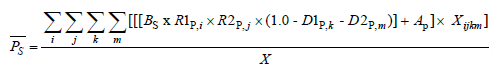Think of if this way: The formula inside the summation is the rating algorithm and represents the total premium for one particular combination of rating variables and discounts. The entire right side of the formula represents the average premium for all combinations of rating variables and discounts. → There are 2 rating variables and 2 discounts. → That's why there are 2+2 = 4 levels of summation. (This is different from the total number of combinations of rating variables and discounts.) (If there had been 3 rating variables and 2 discounts then there would be 3+2 = 5 levels of summation.) (And if all 3 rating variables had 4 levels, plus a binary yes/no for each of 2 discounts, there would be (4x4x4)x(2x2) = 256 combinations of rating variables.)

We're going to look at the 2015.Fall #11 exam problem. The extension of exposures method isn't asked very often, but this question was worth 4 points. (That's a lot of points considering the Exam 5 syllabus says all of Werner Chapter 14 only accounts for 0-3% of the exam.)

E (2015.Fall #11)

The extension of exposures method is kind of a strange method. Here's the question along with the given information. We'll talk through it in general a little bit before presenting the detailed solution, but the only way to really get it into your head is to practice it.

Comments on Alice's solution: (solution is below comments)

• You're told that the average rate should increase by 15%, but you're not given the average rate. To find the current average rate you use extension of exposures, which means to rerate every combination of rating variables. (There are only 2 rating variables and no discounts in this problem.) This is step 1 in Alice's solution below. Once you have the current average rate of $1,012.50, just add 15% to get the proposed average rate of $1,164.38.

• Notice the very sneaky preliminary step of rebasing the proposed relativities. This didn't matter for step 1 because we only needed the current relativities. You will need the rebased proposed relativities in step 2 however or your final answer might be a teensy bit wrong. :-(

• Okay, step 2 is where it gets a bit weird. Remember you're trying to find the proposed base rate, so what do you do? Well, you guess! You just make up any old number then test it to see if it works. This guess for the proposed base rate is called the seed. Alice used $1,000 in her solution. You then use this seed value along with the indicated relativities to calculate the average proposed premium based on this seed. Of course unless you're very lucky, it's not going to be correct. Alice got a "seed" average rate of $691.25, too low, because we're aiming for $1,164.38. You could try another seed, (somewhat higher than $1,000), to see if you get closer but trial and error is a slow way to get the answer.

• Instead of trial and error, you can simply adjust your original guess of $1,000 by an proportionate amount. This is step 3.

• Side comment 1: Something I didn't quite believe when I first read this chapter is that the method will work regardless of what you choose for your seed value. You can use absolutely any random number. You should try it in the Excel spreadsheet. But since it doesn't matter, I always just choose 1.0. Then the seed value just drops out of the calculation entirely. I'm not really sure the concept of seed value is even necessary, but that's the way the text does it so you should probably understand it.

• Side comment 2: The formula used in step 3 uses the proposed fixed expense fee in both the numerator and denominator. At first, I thought this was a misprint in the text but then I realized it's correct because the adjustment is not from the current base rate to the proposed base rate. The adjustment in step 3 is from the seed base rate to the proposed base rate and both the seed and proposed rates use the proposed fixed expense fee. (The current fixed expense fee was used in Step 1 when calculating the current premium.)

Alice's solution:

And here are a couple of practice problems like the above example:

Practice: 2 Extension of Exposure Base Rate problems (like 2015.Fall #11)

Example D: Base Rate - AARD Method

When I read this section in the source text, I was like, huh? Then Alice gave me some advice. :-)

Alice's Pro Tip: The AARD method is easy if you follow her awesome explanation below (even though the text makes it seem mind-numbingly complicated.)

As discussed in the previous section, the extension of exposures method is very accurate but not always feasible because of the detailed data it requires. The AARD method or Approximated Average Rate Differential method is an alternative, but before getting into it I'd like to do a quick review and also mention something I found helpful while reading this chapter. You should keep the goal firmly in mind:

goal: calculate the proposed base rate B_p

In examples B1 and B2, we had 2 versions of a formula for B_p:

• from Example B1:    B_p = B_c x (P_p / P_c)

• from Example B2:    B_p = B_c x (P_p – A_p) / (P_c – A_c)

Example B1 assumed all expenses were variable so a term for fixed expenses wasn't needed. Example B2 did not make the "all variable" assumption. But both B1 and B2 assumed no changes in rate differentials (relativities.)

Example C, which used extension of exposures did allow for changes in rate differentials, and Example D, discussed below, also allows for this. Here's the thing I want to mention: If we temporarily ignore fixed expenses, then the following 3 quantities must balance:

• overall change
• base rate change
• relativity change

If you put these into an equation, you get:

(overall change)   =   (base rate change)   x   (relativity change)

If you think about it for a moment, it's obvious. It follows from the (purely multiplicative) version of the rating algorithm, that is, the version where the fixed expenses are 0. Of course, we can't in general assume that fixed expenses are 0, but I found it helpful to keep in mind this idea of the base rate change and relativity change balancing each other. For a particular overall change, if the base rate change is higher, then the relativity change must be lower, and vice versa. And if you know 2 of these changes, you can calculate the third. That's what this section boils down to. You're typically given the overall change and the relativity changes, then have to calculate the proposed base rate. And a similar way to think about it using premium is:

(proposed premium)   =   (current premium)   x   (base rate change)   x   (relativity change)

It gets slightly messier when you insert fixed expenses but this is the basic idea. Remember this if you find yourself getting confused with all the different formulas and symbols.

Okay, I dunno if all that junk above is helpful to you, but thinking through it like that helped me make more sense of it. If you look at the source text for this section, there is a lot more there than you need to know. If this were a math course where you had to do proofs then you would have to understand it, but that's not the goal here. You only need to learn how to do the calculation, and as Alice said above in her pro-tip, it's actually quite easy. The key concept is S_p:

Sp   =   weighted average proposed rate differential across all rating variables

Then you calculate the proposed base rate B_p using this simple formula:

Bp   =   (Pp – Ap) / Sp

But if you could calculate S_p precisely, then you could use the extension of exposures method. So the AARD method is used in situations where you can't do that. In this case,

approximation to Sp   =   the product of the exposure-weighted average of the rebased indicated relativities

So finally here is Alice's example of AARD using the same numbers from Example C, except that you don't have the same level of detail in the data so you can only get an approximation of S_p.

And here's the solution:

And a couple of practice problems:

Practice: 2 AARD problems

Exam Problems

Problems on calculating a base rate...

mini BattleQuiz 2

Problems on calculating territorial relativities...

mini BattleQuiz 3

Miscellaneous problems...

mini BattleQuiz 4

Full BattleQuiz

POP QUIZ ANSWERS

• A hard market means high prices. (A soft market means low prices)

• Go back